Configure the Viewer
By default, the Rerun Viewer uses heuristics to automatically determine an appropriate layout for your data. However, you'll often want precise control over how your data is displayed. Blueprints give you complete control over the Viewer's layout and configuration.
For a conceptual understanding of blueprints, see Blueprints.
This guide covers three complementary ways to work with blueprints:
- Interactive configuration: Modify layouts directly in the Viewer UI
- Save and load blueprint files: Share layouts using
.rblfiles - Programmatic blueprints: Control layouts from code
Interactive configuration interactive-configuration
The Rerun Viewer is fully configurable through its UI, making it easy to experiment with different layouts.
Viewer overview viewer-overview

The Viewer consists of:
- Viewport (center): Contains your views, arranged in containers
- Blueprint Panel (left): Shows the visual tree of your blueprint structure
- Selection Panel (right): Displays properties of the selected element
- Time Panel (bottom): Controls timeline playback and navigation
The blueprint defines what appears in the viewport. All changes you make to the viewport are actually changes to the blueprint.
Configuring the view hierarchy configuring-the-view-hierarchy
The viewport contains views arranged hierarchically using containers. Containers come in four types:
- Horizontal: Arranges views side-by-side
- Vertical: Stacks views top-to-bottom
- Grid: Organizes views in a grid layout
- Tabs: Shows views in tabs (only one visible at a time)
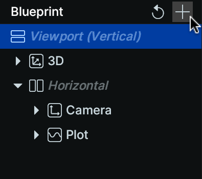
Add new containers or views
Click the "+" button at the top of the blueprint panel to add containers or views.
If a container (or the viewport) is selected, a "+" button also appears in the selection panel.

Rearrange views and containers
Drag and drop items in the blueprint panel to reorganize the hierarchy. You can also drag views directly in the viewport using their title tabs.

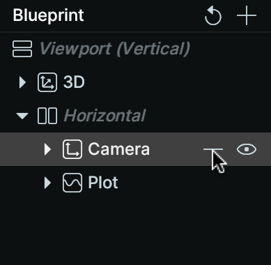
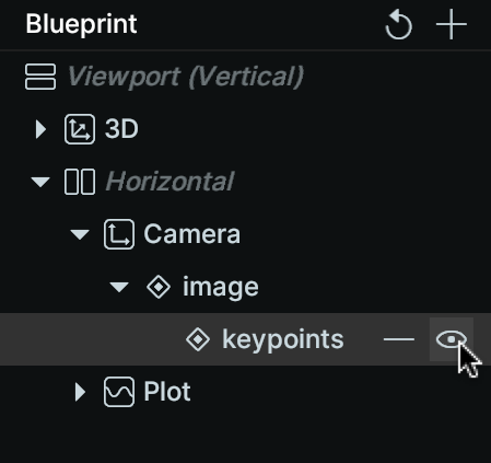
Show, hide, or remove elements
Use the eye icon to show or hide any container, view, or entity:
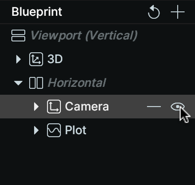
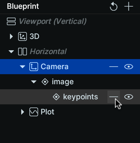
Use the "-" button to permanently remove an element:
Rename views and containers
Select a view or container and edit its name at the top of the selection panel.

Change container type
Select a container and change its type using the dropdown in the selection panel.

Using context menus
Right-click on any element in the blueprint panel for quick access to common operations:
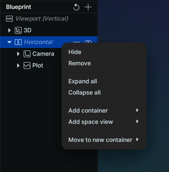
Context menus support multi-selection (Ctrl+click or Cmd+click), enabling bulk operations like removing multiple views at once.
Configuring view content configuring-view-content
Each view displays data based on its entity query. You can modify what appears in a view interactively.
Show or hide entities
Use the eye icon next to any entity to control its visibility within the view.
Remove entities from views
Click the "-" button next to an entity to remove it from the view.
Using the query editor
With a view selected, click "Edit" next to the entity query in the selection panel to visually add or remove entities.

Creating views from entities
Select one or more entities (in existing views or in the time panel's streams), right-click, and choose "Add to new view" from the context menu.

The view's origin will automatically be set based on the selected data.
Overriding visualizers and components overriding-visualizers-and-components
Select an entity within a view to control which visualizers are used and override component values.

When selecting a view, you can also set default component values that apply when no value has been logged.

See Visualizers and Overrides for detailed information.
Save and load blueprint files save-and-load-blueprint-files
Once you've configured your layout, you can save it as a blueprint file (.rbl) to reuse across sessions or share with your team.
Saving a blueprint saving-a-blueprint
To save your current blueprint, go to the file menu and choose "Save blueprint…":
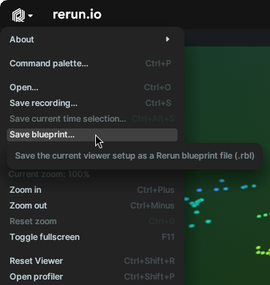
Blueprint files are small, portable, and can be version-controlled alongside your code.
Loading a blueprint loading-a-blueprint
Load a blueprint file using "Open…" from the file menu, or simply drag and drop the .rbl file into the Viewer.
Important: The blueprint's Application ID must match the Application ID of your recording. Blueprints are bound to specific Application IDs to ensure they work with compatible data structures. See Application IDs for more details.
Sharing blueprints sharing-blueprints
Blueprint files make it easy to ensure everyone on your team views data consistently:
- Configure your ideal layout interactively
- Save the blueprint to a
.rblfile - Commit the file to your repository
- Team members load the blueprint when viewing recordings with the same Application ID
This is particularly valuable for:
- Debugging sessions: Share the exact layout needed to diagnose specific issues
- Presentations: Ensure consistent visualization across demos
- Data analysis: Standardize views for comparing results
Programmatic blueprints programmatic-blueprints
For maximum control and automation, you can define blueprints in code using the Python Blueprint API. This is ideal for:
- Creating layouts dynamically based on your data
- Ensuring consistent views for specific debugging scenarios
- Generating complex layouts that would be tedious to build manually
- Sending different blueprints based on runtime conditions
Getting started example getting-started-example
This walkthrough demonstrates the Blueprint API using stock market data. We'll start simple and progressively build more complex layouts.
Setup
First, create a virtual environment and install dependencies:
Linux/Mac:
python -m venv venv
source venv/bin/activate
pip install rerun-sdk humanize yfinance
Windows:
python -m venv venv
.\venv\Scripts\activate
pip install rerun-sdk humanize yfinance
Basic script
Create stocks.py with the necessary imports:
#!/usr/bin/env python3
import datetime as dt
import humanize
import pytz
import yfinance as yf
from typing import Any

import rerun as rr
import rerun.blueprint as rrb
Add helper functions for styling:
brand_colors = {
    "AAPL": 0xA2AAADFF,
    "AMZN": 0xFF9900FF,
    "GOOGL": 0x34A853FF,
    "META": 0x0081FBFF,
    "MSFT": 0xF14F21FF,
}

def style_plot(symbol: str) -> rr.SeriesLine:
    return rr.SeriesLine(
        color=brand_colors[symbol],
        name=symbol,
    )

def style_peak(symbol: str) -> rr.SeriesPoint:
    return rr.SeriesPoint(
        color=0xFF0000FF,
        name=f"{symbol} (peak)",
        marker="Up",
    )

def info_card(
    shortName: str,
    industry: str,
    marketCap: int,
    totalRevenue: int,
    **args: dict[str, Any],
) -> rr.TextDocument:
    markdown = f"""
- **Name**: {shortName}
- **Industry**: {industry}
- **Market cap**: ${humanize.intword(marketCap)}
- **Total Revenue**: ${humanize.intword(totalRevenue)}
"""
    return rr.TextDocument(markdown, media_type=rr.MediaType.MARKDOWN)
Add the main function that logs data:
def main() -> None:
    symbols = ["AAPL", "AMZN", "GOOGL", "META", "MSFT"]

    # Use eastern time for market hours
    et_timezone = pytz.timezone("America/New_York")
    start_date = dt.date(2024, 3, 18)
    dates = [start_date + dt.timedelta(days=i) for i in range(5)]

    # Initialize Rerun and spawn a new viewer
    rr.init("rerun_example_blueprint_stocks", spawn=True)

    # This is where we will edit the blueprint
    blueprint = None
    #rr.send_blueprint(blueprint)

    # Log the stock data for each symbol and date
    for symbol in symbols:
        stock = yf.Ticker(symbol)

        # Log the stock info document as static
        rr.log(f"stocks/{symbol}/info", info_card(**stock.info), static=True)

        for day in dates:
            # Log the styling data as static
            rr.log(f"stocks/{symbol}/{day}", style_plot(symbol), static=True)
            rr.log(f"stocks/{symbol}/peaks/{day}", style_peak(symbol), static=True)

            # Query the stock data during market hours
            open_time = dt.datetime.combine(day, dt.time(9, 30), et_timezone)
            close_time = dt.datetime.combine(day, dt.time(16, 00), et_timezone)

            hist = stock.history(start=open_time, end=close_time, interval="5m")

            # Offset the index to be in seconds since the market open
            hist.index = hist.index - open_time
            peak = hist.High.idxmax()

            # Log the stock state over the course of the day
            for row in hist.itertuples():
                rr.set_time("time", duration=row.Index)
                rr.log(f"stocks/{symbol}/{day}", rr.Scalars(row.High))
                if row.Index == peak:
                    rr.log(f"stocks/{symbol}/peaks/{day}", rr.Scalars(row.High))

if __name__ == "__main__":
    main()
Run the script:
python stocks.pyWithout a blueprint, the heuristic layout may not be ideal:

Creating a simple view creating-a-simple-view
Replace the blueprint section with:
# Create a single chart for all the AAPL data:
blueprint = rrb.Blueprint(
    rrb.TimeSeriesView(name="AAPL", origin="/stocks/AAPL"),
)
rr.send_blueprint(blueprint)
The origin parameter scopes the view to a specific subtree. Now you'll see just the AAPL data:

Controlling panel state controlling-panel-state
You can control which panels are visible:
# Create a single chart and collapse the selection and time panels:
blueprint = rrb.Blueprint(
    rrb.TimeSeriesView(name="AAPL", origin="/stocks/AAPL"),
    rrb.BlueprintPanel(state="expanded"),
    rrb.SelectionPanel(state="collapsed"),
    rrb.TimePanel(state="collapsed"),
)
rr.send_blueprint(blueprint)
Combining multiple views combining-multiple-views
Use containers to combine multiple views. The Vertical container stacks views, and row_shares controls relative sizing:
# Create a vertical layout of an info document and a time series chart
blueprint = rrb.Blueprint(
    rrb.Vertical(
        rrb.TextDocumentView(name="Info", origin="/stocks/AAPL/info"),
        rrb.TimeSeriesView(name="Chart", origin="/stocks/AAPL"),
        row_shares=[1, 4],
    ),
    rrb.BlueprintPanel(state="expanded"),
    rrb.SelectionPanel(state="collapsed"),
    rrb.TimePanel(state="collapsed"),
)
rr.send_blueprint(blueprint)
Specifying view contents specifying-view-contents
The contents parameter provides fine-grained control over what appears in a view. You can include data from multiple sources:
# Create a view with two stock time series
blueprint = rrb.Blueprint(
    rrb.TimeSeriesView(
        name="META vs MSFT",
        contents=[
            "+ /stocks/META/2024-03-19",
            "+ /stocks/MSFT/2024-03-19",
        ],
    ),
    rrb.BlueprintPanel(state="expanded"),
    rrb.SelectionPanel(state="collapsed"),
    rrb.TimePanel(state="collapsed"),
)
rr.send_blueprint(blueprint)
Filtering with expressions filtering-with-expressions
Content expressions can include or exclude subtrees using wildcards. They can reference $origin and use /** to match entire subtrees:
# Create a chart for AAPL and filter out the peaks:
blueprint = rrb.Blueprint(
    rrb.TimeSeriesView(
        name="AAPL",
        origin="/stocks/AAPL",
        contents=[
            "+ $origin/**",
            "- $origin/peaks/**",
        ],
    ),
    rrb.BlueprintPanel(state="expanded"),
    rrb.SelectionPanel(state="collapsed"),
    rrb.TimePanel(state="collapsed"),
)
rr.send_blueprint(blueprint)
See Entity Queries for complete expression syntax.
Programmatic layout generation programmatic-layout-generation
Since blueprints are Python code, you can generate them dynamically. This example creates a grid with one row per stock symbol:
# Iterate over all symbols and days to create a comprehensive grid
blueprint = rrb.Blueprint(
    rrb.Vertical(
        contents=[
            rrb.Horizontal(
                contents=[
                    rrb.TextDocumentView(
                        name=f"{symbol}",
                        origin=f"/stocks/{symbol}/info",
                    ),
                ]
                + [
                    rrb.TimeSeriesView(
                        name=f"{day}",
                        origin=f"/stocks/{symbol}/{day}",
                    )
                    for day in dates
                ],
                name=symbol,
            )
            for symbol in symbols
        ]
    ),
    rrb.BlueprintPanel(state="expanded"),
    rrb.SelectionPanel(state="collapsed"),
    rrb.TimePanel(state="collapsed"),
)
rr.send_blueprint(blueprint)
Saving blueprints from code saving-blueprints-from-code
You can save programmatically-created blueprints to .rbl files:
blueprint = rrb.Blueprint(
    rrb.TimeSeriesView(name="AAPL", origin="/stocks/AAPL"),
)

# Save to a file
blueprint.save("rerun_example_blueprint_stocks", "my_blueprint.rbl")

# Later, load it in any language
rr.log_file_from_path("my_blueprint.rbl")
This enables reusing blueprints across different programming languages. See the Blueprint API Reference for complete details.
Advanced customization advanced-customization
Blueprints support deep customization of view properties. For example:
# Configure a 3D view with custom camera settings
rrb.Spatial3DView(
    name="Robot view",
    origin="/world/robot",
    background=[100, 149, 237],  # Light blue
    eye_controls=rrb.EyeControls3D(
        kind=rrb.Eye3DKind.FirstPerson,
        speed=20.0,
    ),
)

# Configure a time series view with custom axis and time ranges
rrb.TimeSeriesView(
    name="Sensor Data",
    origin="/sensors",
    axis_y=rrb.ScalarAxis(range=(-10.0, 10.0), zoom_lock=True),
    plot_legend=rrb.PlotLegend(visible=False),
    time_ranges=[
        rrb.VisibleTimeRange(
            "time",
            start=rrb.TimeRangeBoundary.cursor_relative(seq=-100),
            end=rrb.TimeRangeBoundary.cursor_relative(),
        ),
    ],
)
See Visualizers and Overrides for information on overriding component values and controlling visualizers from code.
Youtube overview youtube-overview
While some people might want to read through the documentation on this page, others might prefer to watch a video! If you would like to follow along with the Youtube video, you can find the code used in the video below.
from __future__ import annotations

import math

import numpy as np
import rerun as rr
import rerun.blueprint as rrb
from numpy.random import default_rng

rr.init("rerun_blueprint_example", spawn=True)

rr.set_time("time", sequence=0)
rr.log("log/status", rr.TextLog("Application started.", level=rr.TextLogLevel.INFO))
rr.set_time("time", sequence=5)
rr.log("log/other", rr.TextLog("A warning.", level=rr.TextLogLevel.WARN))
for i in range(10):
    rr.set_time("time", sequence=i)
    rr.log(
        "log/status", rr.TextLog(f"Processing item {i}.", level=rr.TextLogLevel.INFO)
    )

# Create a text view that displays all logs.
blueprint = rrb.Blueprint(
    rrb.TextLogView(origin="/log", name="Text Logs"),
    rrb.SelectionPanel(state="expanded"),
    collapse_panels=True,
)

rr.send_blueprint(blueprint)


input("Press Enter to continue…")

# Create a spiral of points:
n = 150
angle = np.linspace(0, 10 * np.pi, n)
spiral_radius = np.linspace(0.0, 3.0, n) ** 2
positions = np.column_stack(
    (np.cos(angle) * spiral_radius, np.sin(angle) * spiral_radius)
)
colors = np.dstack(
    (np.linspace(255, 255, n), np.linspace(255, 0, n), np.linspace(0, 255, n))
)[0].astype(int)
radii = np.linspace(0.01, 0.7, n)

rr.log("points", rr.Points2D(positions, colors=colors, radii=radii))

# Create a Spatial2D view to display the points.
blueprint = rrb.Blueprint(
    rrb.Spatial2DView(
        origin="/",
        name="2D Scene",
        # Set the background color
        background=[105, 20, 105],
        # Note that this range is smaller than the range of the points,
        # so some points will not be visible.
        visual_bounds=rrb.VisualBounds2D(x_range=[-5, 5], y_range=[-5, 5]),
    ),
    collapse_panels=True,
)

rr.send_blueprint(blueprint)


input("Press Enter to continue…")

rr.log(
    "points",
    rr.GeoPoints(
        lat_lon=[[47.6344, 19.1397], [47.6334, 19.1399]],
        radii=rr.Radius.ui_points(20.0),
    ),
)

# Create a map view to display the chart.
blueprint = rrb.Blueprint(
    rrb.MapView(
        origin="points",
        name="MapView",
        zoom=16.0,
        background=rrb.MapProvider.OpenStreetMap,
    ),
    collapse_panels=True,
)


rr.send_blueprint(blueprint)

input("Press Enter to continue…")

blueprint = rrb.Blueprint(
    rrb.Grid(
        rrb.MapView(
            origin="points",
            name="MapView",
            zoom=16.0,
            background=rrb.MapProvider.OpenStreetMap,
        ),
        rrb.Spatial2DView(
            origin="/",
            name="2D Scene",
            # Set the background color
            background=[105, 20, 105],
            # Note that this range is smaller than the range of the points,
            # so some points will not be visible.
            visual_bounds=rrb.VisualBounds2D(x_range=[-5, 5], y_range=[-5, 5]),
        ),
        rrb.TextLogView(origin="/log", name="Text Logs"),
    ),
    rrb.TimePanel(state="expanded"),
    rrb.BlueprintPanel(state="expanded"),
    collapse_panels=True,
)

rr.send_blueprint(blueprint)

blueprint.save("my_favorite_blueprint", "data/blueprint.rbl")

input("Press Enter to continue…")


rr.log("bar_chart", rr.BarChart([8, 4, 0, 9, 1, 4, 1, 6, 9, 0]))

rng = default_rng(12345)
positions = rng.uniform(-5, 5, size=[50, 3])
colors = rng.uniform(0, 255, size=[50, 3])
radii = rng.uniform(0.1, 0.5, size=[50])

rr.log("3dpoints", rr.Points3D(positions, colors=colors, radii=radii))

tensor = np.random.randint(0, 256, (32, 240, 320, 3), dtype=np.uint8)
rr.log("tensor", rr.Tensor(tensor, dim_names=("batch", "x", "y", "channel")))

rr.log(
    "markdown",
    rr.TextDocument(
        """
# Hello Markdown!
[Click here to see the raw text](recording://markdown:Text).
"""
    ),
)

rr.log("trig/sin", rr.SeriesLines(colors=[255, 0, 0], names="sin(0.01t)"), static=True)
for t in range(int(math.pi * 4 * 100.0)):
    rr.set_time("time", sequence=t)
    rr.set_time("timeline1", duration=t)
    rr.log("trig/sin", rr.Scalars(math.sin(float(t) / 100.0)))

blueprint = rrb.Blueprint(
    rrb.Grid(
        rrb.MapView(
            origin="points",
            name="MapView",
            zoom=16.0,
            background=rrb.MapProvider.OpenStreetMap,
        ),
        rrb.Spatial2DView(
            origin="/",
            name="2D Scene",
            # Set the background color
            background=[105, 20, 105],
            # Note that this range is smaller than the range of the points,
            # so some points will not be visible.
            visual_bounds=rrb.VisualBounds2D(x_range=[-5, 5], y_range=[-5, 5]),
        ),
        rrb.TextLogView(origin="/log", name="Text Logs"),
        rrb.BarChartView(origin="bar_chart", name="Bar Chart"),
        rrb.Spatial3DView(
            origin="/3dpoints",
            name="3D Scene",
            # Set the background color to light blue.
            background=[100, 149, 237],
            # Configure the eye controls.
            eye_controls=rrb.EyeControls3D(
                kind=rrb.Eye3DKind.FirstPerson,
                speed=20.0,
            ),
        ),
        rrb.TensorView(
            origin="tensor",
            name="Tensor",
            # Explicitly pick which dimensions to show.
            slice_selection=rrb.TensorSliceSelection(
                # Use the first dimension as width.
                width=1,
                # Use the second dimension as height and invert it.
                height=rr.TensorDimensionSelection(dimension=2, invert=True),
                # Set which indices to show for the other dimensions.
                indices=[
                    rr.TensorDimensionIndexSelection(dimension=2, index=4),
                    rr.TensorDimensionIndexSelection(dimension=3, index=5),
                ],
                # Show a slider for dimension 2 only. If not specified, all dimensions in `indices` will have sliders.
                slider=[2],
            ),
            # Set a scalar mapping with a custom colormap, gamma and magnification filter.
            scalar_mapping=rrb.TensorScalarMapping(
                colormap="turbo", gamma=1.5, mag_filter="linear"
            ),
            # Fill the view, ignoring aspect ratio.
            view_fit="fill",
        ),
        rrb.TextDocumentView(origin="markdown", name="Markdown example"),
        rrb.TimeSeriesView(
            origin="/trig",
            # Set a custom Y axis.
            axis_y=rrb.ScalarAxis(range=(-1.0, 1.0), zoom_lock=True),
            # Configure the legend.
            plot_legend=rrb.PlotLegend(visible=False),
            # Set time different time ranges for different timelines.
            time_ranges=[
                # Sliding window depending on the time cursor for the first timeline.
                rrb.VisibleTimeRange(
                    "time",
                    start=rrb.TimeRangeBoundary.cursor_relative(seq=-100),
                    end=rrb.TimeRangeBoundary.cursor_relative(),
                ),
                # Time range from some point to the end of the timeline for the second timeline.
                rrb.VisibleTimeRange(
                    "timeline1",
                    start=rrb.TimeRangeBoundary.absolute(seconds=300.0),
                    end=rrb.TimeRangeBoundary.infinite(),
                ),
            ],
        ),
    ),
    collapse_panels=True,
)

rr.send_blueprint(blueprint)
Next steps next-steps
- Explore view types: Check the View Type Reference to see all available views and their configuration options
- Learn about overrides: See Visualizers and Overrides for per-entity customization
- API Reference: Browse the complete Blueprint API for programmatic control